What the measurement actually means
A projection zone boundary is an administrative division of a coordinate system family, not a physical discontinuity in the landscape. Data on opposite sides can still be analyzed together in an appropriate common CRS. Problems arise when coordinates from different zones are merged as though they shared one plane, or when automatic transformations hide inconsistent assumptions. The choice of a common projection should consider the full extent, distortion, intended measurements, and existing survey requirements rather than simply choosing whichever zone appears first in a folder.
A reproducible working procedure
Inventory the native CRS of every tile and control dataset before merging. Select a common output CRS with an appropriate area of use and inspect its scale behavior across the footprint. Transform the sources explicitly, keeping their original definitions in the manifest. For a raster mosaic, also establish one resolution, origin, and alignment. For vector measurements, verify the calculation method and units. Compare overlaps near the boundary using common physical features and independently known coordinates where available.
Illustrative calculation and interpretation
Imagine an illustrative corridor extending twenty kilometres west and twenty kilometres east of a nominal zone boundary. Eastings from the two native zones cannot be concatenated as one continuous axis because their central meridians and false origins differ. A common projection may serve the forty kilometre corridor adequately, but that must be evaluated against the required measurement tolerance. If a local scale departure is 200 parts per million, a one kilometre grid distance differs by about 0.2 metres from the corresponding reference scale under the simplified comparison.
Quality checks and failure diagnosis
Inspect seam alignment numerically and visually after transformation, keeping projection distortion separate from image registration error. Test a known line crossing the boundary rather than checking only within each original tile. Do not correct a seam by manually translating one zone dataset until the coordinate definitions and operations have been verified. Record why the chosen common CRS is acceptable and any remaining ground to grid considerations. This allows a receiving analyst to continue measurements without reconstructing the logic from filenames or map screenshots.
Start with an explicit data contract
Write down the intended geometry or raster meaning, coordinate reference system, horizontal and vertical units, extent, and required attributes before conversion. Keep the source file unchanged and create a small representative test area containing both ordinary features and awkward edges. This makes it possible to verify the operation quickly while retaining cases that expose real failures. A successful file opening is only a readability check; it does not demonstrate that the numbers, coordinate interpretation, or feature semantics survived the transfer.
Inspect numbers as well as appearance
Read the metadata and sample actual coordinates or cell values in addition to viewing a styled map. On the fly reprojection, automatic contrast stretching, and hidden null values can make incompatible datasets appear convincing. Record the native bounds, dimensions, field definitions, and a few stable sample records before processing. Repeat the same checks afterward. Keep the display settings separate from analytical values so that a change in color ramp or scale cannot be mistaken for a change in the underlying geographic measurement.
Use a reversible processing sequence
Build the workflow from explicit steps with named intermediate outputs and record the options used at each step. Test the smallest meaningful subset first, then apply the validated sequence to the full extent. Avoid overwriting inputs during experiments. Where an operation changes coordinates, resolution, geometry, or numeric type, state that change in the processing note. Reversibility helps diagnosis, but it does not imply that a lossy operation can recover its original detail; keep the unmodified source for that reason.
Validate spatially and numerically
Compare source and output at interior locations, boundaries, and areas with missing data. Check both global summaries and local samples because opposite errors can cancel in a mean. For vectors, inspect feature counts, identifiers, and geometry validity; for rasters, inspect band statistics, masks, grid dimensions, and sampled values. If a result differs, classify whether the difference is intended, a rounding consequence, or a defect. Keep evidence for representative locations rather than relying on a single whole map screenshot.
Carry uncertainty into downstream use
The number of stored decimal places is a storage choice, not a measurement accuracy statement. Preserve the uncertainty and resolution of the source separately from the precision of its encoding. When an operation interpolates, generalizes, or aggregates, describe the new support area and any assumptions about values between observations. A later analysis should not treat every newly created vertex or pixel as an independent field observation. This distinction matters particularly when calculating areas, distances, surface differences, or statistics over small management units.
Make the handover self describing
Deliver the data with a concise manifest identifying its source, creation date, coordinate system, units, processing history, and known limitations. Include the software version and any auxiliary resources needed to interpret it. Reopen the exported file in a separate reader where practical, then verify several named test features or coordinates against the source. A clean handover allows another analyst to reproduce the intended interpretation and prevents a future conversion from quietly replacing a documented assumption with a convenient application default.
Test the decision, not just the file
Define the downstream decision before choosing an acceptance tolerance. An overview map, a repeat survey comparison, and an engineering measurement can use similar looking files while requiring different evidence. Write the tolerance in physical units and state the footprint where it applies. If the available checks do not cover a surface type or operating condition, identify that gap explicitly. This makes a conditional acceptance useful: the analyst can release a supported portion, retain a flagged portion for investigation, and avoid silently extending evidence beyond the locations actually examined.
Distinguish an assumption from an observation
Keep a short interpretation note separating measured quantities, calculations, and assumptions. The numerical example in this article is an illustration of a mechanism; replace its inputs with project measurements before making an operational decision. For an uncertain input, repeat the calculation over a defensible range and see whether the conclusion changes. If it does, obtaining better evidence for that input may be more valuable than adjusting unrelated processing settings. Retain the alternative results so a reviewer can understand why the selected workflow was judged adequate.
Using the result in a mapping project
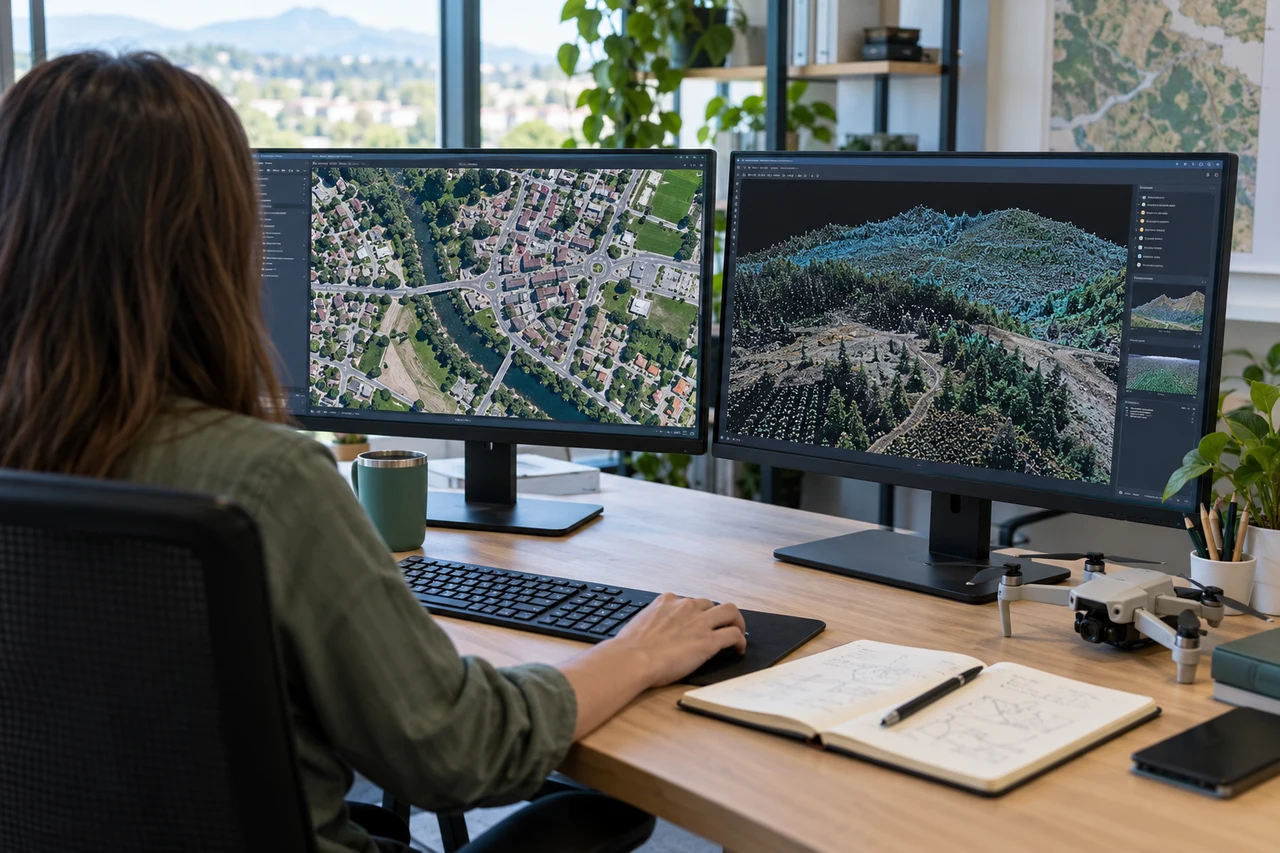
Online Photogrammetry Software is most useful here when its outputs remain connected to the documented inputs and checks. A DroneCollab project can be considered as one processing destination, while the analyst retains responsibility for coordinate interpretation, independent validation, and suitability for the intended measurement. Confirm the available import and export options for the actual project rather than assuming that a product name establishes support or accuracy.